File:SimudoyaTb.png

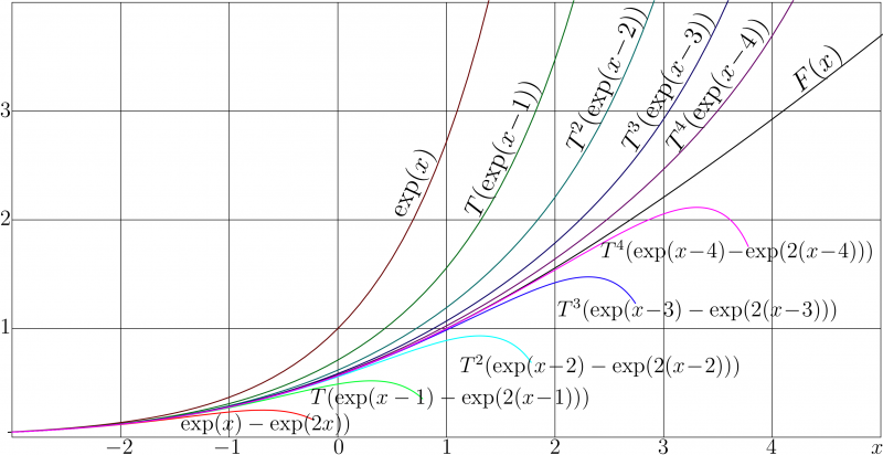
Recovery of superfunction of the transfer function

\(T=\ \)Doya\(_1\) by the Regular iteration method.

\(T\) can be expressed also through the LambertW function:

\(T(z)=\mathrm{Doya}_1(z)=\mathrm{LambertW}\Big( z~ \mathrm{e}^{z+1} \Big)\)

\(T\) can be interpreted as a transfer function of the idealized laser amplifier.
Its superfunction \(F\) describes the evolution of the normalized intensity along the direction of amplification.

The brown curve and the red curve represent the primary approximations of \(F\) with one term and with two terms of the asymptotic expansion, respectively.

Green, cyan, blue and magenta curves represent the First, Second, Third and Fourth iteration of the approximation with 2 terms; the curves of corresponding dark colors represent the regular iterations of the primary approximation with single term.

For this example of the transfer function, the analytic representation of the superfunction \(F\) through the Tania function exist:

\[ F(x)=\mathrm{Tania}(x\!-\!1)=\mathrm{LambertW}(\exp(x)) \]

This superfunction is plotted with black curve.

The primary approximations show good agreement while argument \(x\!<\!-2\); for larger values of \(x\), transfer function \(T\) should be iterated, roughtly, \(n=x\!+\!2\) times, misplacing the argument for $\(n\); id est, \[ F(x)\approx T^n( \tilde F (x\!-\!n))\]

Here \(\tilde F\) is one of the primary approximations.

Superfunctions

The explicit plot above appears as Fig.6.2 at page 66 of book «Superfunctions» ^[1][2]
in order to show how the regular iteration works, using the simple example with the easy transfer function that allows to trace each step of the evaluation of the superfunction.

C++ generator of curves

// FIles ado.cin and doya.cin should be loaded to the current directory in order to compile the C++ code below:

#include <math.h>
#include <stdio.h>
#include <stdlib.h>
#define DB double
#define DO(x,y) for(x=0;x<y;x++)
using namespace std;
#include <complex>
typedef complex<double> z_type;
#define Re(x) x.real()
#define Im(x) x.imag()
#define I z_type(0.,1.)
DB ArcTania(DB x){ return x+log(x)-1.;}
#include "ado.cin"
#include "doya.cin"
#define M(x,y) fprintf(o,"%6.4f %6.4f M\n",0.+x,0.+y);
#define L(x,y) fprintf(o,"%6.4f %6.4f L\n",0.+x,0.+y);
main(){ int j,k,m,n; DB x,y,t,e, a; z_type z;
FILE *o;o=fopen("simudoya.eps","w");ado(o,808,408);
fprintf(o,"404 4 translate\n 100 100 scale\n");
for(m=-4;m<5;m++){ M(m,0)L(m,4)}
for(n=0;n<5;n++){ M(-4,n)L(4,n)}
fprintf(o,"2 setlinecap\n");
fprintf(o,".006 W 0 0 0 RGB S\n");
fprintf(o,"1 setlinejoin 1 setlinecap\n");
// for(n=0;n<380;n++){y=.02+.01*n; x=ArcTania(y); if(n==0)M(x,y) else L(x,y)} fprintf(o,".03 W 0 1 0 RGB S\n");
for(n=0;n<82;n++){x=-4.05+.1*n;z=x;y=Re(Tania(z)); if(n==0)M(x,y) else L(x,y)} fprintf(o,".01 W 0 0 0 RGB S\n");
//
for(n=0;n<45;n++){x=-4+.1*n;e=exp(x+1.); y=e;                       ; if(n==0)M(x,y) else L(x,y)} fprintf(o,".01 W .4 0 0 RGB S\n");
for(n=0;n<70;n++){x=-4+.04*n;e=exp(x+1.); y=e*(1.-e);                ; if(n==0)M(x,y) else L(x,y)} fprintf(o,".01 W 1 0 0 RGB S\n");
//
for(n=0;n<53;n++){x=-4+.1*n;e=exp(x+0.); y=e       ; y=Re(Doya(1.,y));if(n==0)M(x,y) else L(x,y)} fprintf(o,".01 W 0 .4 0 RGB S\n");
for(n=0;n<190;n++){x=-4+.02*n;e=exp(x+0.); y=e*(1.-e); y=Re(Doya(1.,y));if(n==0)M(x,y) else L(x,y)} fprintf(o,".01 W 0 1 0 RGB S\n");
//
for(n=0;n<61;n++){x=-4+.1*n;e=exp(x-1.); y=e       ;DO(m,2)y=Re(Doya(1.,y));if(n==0)M(x,y) else L(x,y)} fprintf(o,".01 W 0 .4 0.4 RGB S\n");
for(n=0;n<240;n++){x=-4+.02*n;e=exp(x-1.); y=e*(1.-e);DO(m,2)y=Re(Doya(1.,y));if(n==0)M(x,y) else L(x,y)} fprintf(o,".01 W 0 1 1 RGB S\n");
//
for(n=0;n<67;n++){x=-4+.1*n;e=exp(x-2.); y=e       ;DO(m,3)y=Re(Doya(1.,y));if(n==0)M(x,y) else L(x,y)} fprintf(o,".01 W 0 0 0.4 RGB S\n");
for(n=0;n<288;n++){x=-4+.02*n;e=exp(x-2.); y=e*(1.-e);DO(m,3)y=Re(Doya(1.,y));if(n==0)M(x,y) else L(x,y)} fprintf(o,".01 W 0 0 1 RGB S\n");
//
for(n=0;n<73;n++){x=-4+.1*n;e=exp(x-3.); y=e       ;DO(m,4)y=Re(Doya(1.,y));if(n==0)M(x,y) else L(x,y)} fprintf(o,".01 W .4 0 0.4 RGB S\n");
for(n=0;n<340;n++){x=-4+.02*n;e=exp(x-3.); y=e*(1.-e);DO(m,4)y=Re(Doya(1.,y));if(n==0)M(x,y) else L(x,y)} fprintf(o,".01 W 1 0 1 RGB S\n");
//
fprintf(o,"showpage\n%cTrailer",'%'); fclose(o);
       system("epstopdf simudoya.eps");
       system(    "open simudoya.pdf"); //these 2 commands may be specific for macintosh
getchar(); system("killall Preview");// if run at another operational sysetm, may need to modify
}

Latex generator of labels

File simudoya.pdf should be generated with the code above in order to compile the Latex document below.

\documentclass[12pt]{article} %<br>
\usepackage{geometry}  %<br>
\usepackage{graphicx} %<br>
\usepackage{hyperref} %<br>
\usepackage{rotating} %<br>
\paperwidth  1632pt %<br>
\paperheight 840pt %<br>
\topmargin -102pt %<br>
\oddsidemargin -58pt %<br>
\textwidth 1825pt %<br>
\textheight 1470pt %<br>
\newcommand \sx {\scalebox} %<br>
\newcommand \ing {\includegraphics} %<br>
\newcommand \tet {\mathrm{tet}} %<br>
\newcommand \pen {\mathrm{pen}} %<br>
\newcommand \bC {\mathbb C} %<br>
\newcommand \fac {\mathrm {Factorial}} %<br>
\newcommand \rme {\mathrm e} %<br>
\newcommand \rmi {\mathrm i} %<br>
\newcommand \ds {\displaystyle} %<br>
\newcommand \rot {\begin{rotate}} %<br>
\newcommand \ero {\end{rotate}} %<br>
\pagestyle{empty} %<br>
\begin{document} %<br>
\parindent 0pt %<br>
\sx{2}{\begin{picture}(600,404) %<br>
\put(0,0){\ing{simudoya}} %<br>
\put(-7,300){\sx{1.7}{$3$}} %<br>
\put(-7,200){\sx{1.7}{$2$}} %<br>
\put(-7,100){\sx{1.7}{$1$}} %<br>
\put(90,-11){\sx{1.7}{$-2$}} %<br>
\put(190,-11){\sx{1.7}{$-1$}} %<br>
\put(301,-11){\sx{1.7}{$0$}} %<br>
\put(401,-11){\sx{1.7}{$1$}} %<br>
\put(501,-11){\sx{1.7}{$2$}} %<br>
\put(601,-11){\sx{1.7}{$3$}} %<br>
\put(701,-11){\sx{1.7}{$4$}} %<br>
\put(798,-11){\sx{1.7}{$x$}} %<br>
\put(366,206){\rot{65}\sx{2}{$\exp(x)$}\ero} %<br>
\put(436,206){\rot{66}\sx{2}{$T(\exp(x\!-\!1))$}\ero} %<br>
\put(530,266){\rot{66}\sx{2}{$T^2(\exp(x\!-\!2))$}\ero} %<br>
\put(580,266){\rot{60}\sx{2}{$T^3(\exp(x\!-\!3))$}\ero} %<br>
\put(620,266){\rot{55}\sx{2}{$T^4(\exp(x\!-\!4))$}\ero} %<br>
\put(733,322){\rot{41}\sx{2.1}{$F(x)$}\ero} %<br>
\put(548,170){\sx{1.7}{$T^4(\exp(x\!-\!4)\!-\!\exp(2(x\!-\!4)))$}} %<br>
\put(508,116){\sx{1.7}{$T^3(\exp(x\!-\!3)-\exp(2(x\!-\!3)))$}} %<br>
\put(418,64){\sx{1.7}{$T^2(\exp(x\!-\!2)-\exp(2(x\!-\!2)))$}} %<br>
\put(280,35){\sx{1.7}{$T(\exp(x-1)-\exp(2(x\!-\!1)))$}} %<br>
\put(160,11){\sx{1.7}{$\exp(x)-\exp(2x))$}} %<br>
\end{picture}} %<br>
\end{document} %<br>
%

References

Keywords

«ArcTania», «Doya function», «Tania function», «Superfunction»,

References

- ↑ https://www.amazon.co.jp/Superfunctions-Non-integer-holomorphic-functions-superfunctions/dp/6202672862 Dmitrii Kouznetsov. Superfunctions: Non-integer iterates of holomorphic functions. Tetration and other superfunctions. Formulas,algorithms,tables,graphics - 2020/7/28
- ↑ https://mizugadro.mydns.jp/BOOK/468.pdf Dmitrii Kouznetsov (2020). Superfunctions: Non-integer iterates of holomorphic functions. Tetration and other superfunctions. Formulas, algorithms, tables, graphics. Publisher: Lambert Academic Publishing.