Difference between revisions of "File:Expe1eplotT.jpg"
($ -> \( ; description ; refs ; pre ; keywords) |
|||
| Line 1: | Line 1: | ||
| + | {{oq|Expe1eplotT.jpg|Original file (2,515 × 1,751 pixels, file size: 350 KB, MIME type: image/jpeg) }} |
||
| + | |||
[[Explicit plot]] of [[exponential]] to [[base e1e]] (thick green curve) and |
[[Explicit plot]] of [[exponential]] to [[base e1e]] (thick green curve) and |
||
that of the [[exponential]] to [[base sqrt2]] (thin red curve) |
that of the [[exponential]] to [[base sqrt2]] (thin red curve) |
||
| − | Here, |
+ | Here, \(\eta\!=\!\exp(1/\mathrm e)\!\approx1.44466786 \ \) is the [[Henryk base]]. At this base, the exponential has only one real [[fixed point]], |
| − | id est, equation |
+ | id est, equation \(\exp_\eta(L)\!=\!L\) has only one real solution \(L\!=\!\mathrm e\!\approx\! 2.71~\) and \(\ \exp_{\eta}^{\ \prime}(L)\!=\!1\ \). Henryk Trappmann had expected, for this base, the [[superexponential]] is very interesting because it is very difficult to construct, if at al. However, it happened to be not so <ref> |
| + | http://www.ams.org/journals/mcom/0000-000-00/S0025-5718-2012-02590-7/S0025-5718-2012-02590-7.pdf <br> |
||
| + | https://mizugadro.mydns.jp/PAPERS/2012e1eMcom2590.pdf |
||
| + | H.Trappmann, D.Kouznetsov. Computation of the Two Regular Super-Exponentials to base exp(1/e). Mathematics of Computation. Math. Comp., v.81 (2012), p. 2207-2227. ISSN 1088-6842(e) ISSN 0025-5718(p) |
||
| + | </ref>. |
||
| − | The thick green curve is |
+ | The thick green curve is \(\ y\!=\!\eta^x\ \). |
| − | In order to show the fixed point, the thin line |
+ | In order to show the fixed point, the thin line \(\ y\!=\!x\ \) is drawn. |
| − | For comparison, the exponential to base |
+ | For comparison, the exponential to base \(\ b\!=\! \sqrt{2}\ \) is plotted, that has two fixed points, \(\ L\!=\!2\ \) and \(\ L\!=\!4\ \). |
==[[C++]] generator of curves== |
==[[C++]] generator of curves== |
||
| + | //<pre> |
||
| − | //<poem><nomathjax><nowiki> |
||
#include<math.h> |
#include<math.h> |
||
#include<stdio.h> |
#include<stdio.h> |
||
| Line 42: | Line 48: | ||
getchar(); system("killall Preview");//for mac |
getchar(); system("killall Preview");//for mac |
||
} |
} |
||
| + | //</pre> |
||
| − | //</nowiki></nomathjax></poem> |
||
==[[Latex]] generator of labels== |
==[[Latex]] generator of labels== |
||
| + | %<pre> |
||
| − | %<poem><nomathjax><nowiki> |
||
\documentclass[12pt]{article} |
\documentclass[12pt]{article} |
||
\usepackage{geometry} |
\usepackage{geometry} |
||
| Line 96: | Line 102: | ||
\end{picture}} |
\end{picture}} |
||
\end{document} |
\end{document} |
||
| + | </pre> |
||
| − | </nowiki></nomathjax></poem> |
||
| + | ==References== |
||
| ⚫ | |||
| + | {{ref}} |
||
| ⚫ | |||
| + | |||
| + | {{fer}} |
||
| + | |||
| + | ==Keywords== |
||
| + | |||
| + | «[[Base e1e]]», |
||
| + | «[[Base sqrt2]]», |
||
| + | «[[Exotic iteration]]», |
||
| + | «[[Exp]]», |
||
| + | «[[Superfunctions]]», |
||
| + | «[[]]», |
||
| ⚫ | |||
| + | «[[]]», |
||
| + | |||
| + | [[Category:Abelfunction]] |
||
[[Category:Base e1e]] |
[[Category:Base e1e]] |
||
[[Category:Base sqrt2]] |
[[Category:Base sqrt2]] |
||
| ⚫ | |||
| ⚫ | |||
| ⚫ | |||
| ⚫ | |||
| ⚫ | |||
[[Category:Exponential]] |
[[Category:Exponential]] |
||
[[Category:Fixed point]] |
[[Category:Fixed point]] |
||
| ⚫ | |||
| ⚫ | |||
| ⚫ | |||
| ⚫ | |||
| ⚫ | |||
[[Category:Latex]] |
[[Category:Latex]] |
||
| + | [[Category:Transfer function]] |
||
| + | [[Category:Superfunction]] |
||
| + | [[Category:Superfunctions]] |
||
Revision as of 15:42, 23 August 2025
Explicit plot of exponential to base e1e (thick green curve) and that of the exponential to base sqrt2 (thin red curve)
Here, \(\eta\!=\!\exp(1/\mathrm e)\!\approx1.44466786 \ \) is the Henryk base. At this base, the exponential has only one real fixed point, id est, equation \(\exp_\eta(L)\!=\!L\) has only one real solution \(L\!=\!\mathrm e\!\approx\! 2.71~\) and \(\ \exp_{\eta}^{\ \prime}(L)\!=\!1\ \). Henryk Trappmann had expected, for this base, the superexponential is very interesting because it is very difficult to construct, if at al. However, it happened to be not so [1].
The thick green curve is \(\ y\!=\!\eta^x\ \).
In order to show the fixed point, the thin line \(\ y\!=\!x\ \) is drawn.
For comparison, the exponential to base \(\ b\!=\! \sqrt{2}\ \) is plotted, that has two fixed points, \(\ L\!=\!2\ \) and \(\ L\!=\!4\ \).
C++ generator of curves
//#include<math.h>
#include<stdio.h>
#include<stdlib.h>
#define DB double
#define DO(x,y) for(x=0;x<y;x++)
#include "ado.cin"
DB B=sqrt(2.);
int main(){ int m,n; double x,y; FILE *o;
o=fopen("expe1eplot.eps","w"); ado(o,1204,804);
fprintf(o,"602 2 translate 100 100 scale\n");
#define M(x,y) fprintf(o,"%6.3f %6.3f M\n",0.+x,0.+y);
#define L(x,y) fprintf(o,"%6.3f %6.3f L\n",0.+x,0.+y);
for(m=-6;m<7;m++) {M(m,0)L(m,8)}
for(m=0;m<9;m++) {M(-6,m)L(6,m)}
fprintf(o,"2 setlinecap .01 W S\n 1 setlinejoin \n");
M(M_E,0)L(M_E,M_E)L(0,M_E) fprintf(o,".007 W S\n");
for(m=0;m<123;m++){x=-6.1+.1*m; y=exp(log(B)*x); if(m==0)M(x,y) else L(x,y);} fprintf(o,".02 W .8 0 0 RGB S\n");
for(m=0;m<123;m++){x=-6.1+.1*m; y=exp(x/M_E); if(m==0)M(x,y) else L(x,y);} fprintf(o,".04 W 0 .6 0 RGB S\n");
M(-.1,-.1)L(6.1,6.1) fprintf(o,".016 W 0 0 0 RGB S\n\n");
fprintf(o,"showpage\n%c%cTrailer",'%','%'); fclose(o);
system("epstopdf expe1eplot.eps");
system( "open expe1eplot.pdf");
getchar(); system("killall Preview");//for mac
}
//
Latex generator of labels
%\documentclass[12pt]{article}
\usepackage{geometry}
\usepackage{graphicx}
\usepackage{rotating}
\paperwidth 1212pt
\paperheight 844pt
\topmargin -92pt
\oddsidemargin -80pt
\textwidth 1604pt
\textheight 1604pt
\pagestyle {empty}
\newcommand \sx {\scalebox}
\newcommand \rot {\begin{rotate}}
\newcommand \ero {\end{rotate}}
\newcommand \ing {\includegraphics}
\parindent 0pt
\pagestyle{empty}
\begin{document}
{\begin{picture}(1202,802)
\put(590,792){\sx{4.2}{$y$}}
\put(590,698){\sx{4.2}{$7$}}
\put(590,598){\sx{4.2}{$6$}}
\put(590,498){\sx{4.2}{$5$}}
\put(590,398){\sx{4.2}{$4$}}
\put(590,298){\sx{4.2}{$3$}}
\put(620,274){\sx{4.2}{$\mathrm e$}}
\put(590,198){\sx{4.2}{$2$}}
\put(590,098){\sx{4.2}{$1$}}
\put(080,-22){\sx{4}{$-5$}}
\put(180,-22){\sx{4}{$-4$}}
\put(281,-22){\sx{4}{$-3$}}
\put(381,-22){\sx{4}{$-2$}}
\put(482,-22){\sx{4}{$-\!1$}}
\put(603.6,-22){\sx{4}{$0$}}
\put(703.7,-22){\sx{4}{$1$}}
\put(803.8,-22){\sx{4}{$2$}}
\put(877.,16){\sx{4}{$\mathrm e$}}
\put(903.9,-22){\sx{4}{$3$}}
\put(1004.0,-22){\sx{4}{$4$}}
\put(1104.1,-22){\sx{4}{$5$}}
\put(1192.2,-22){\sx{4.3}{$x$}}
%\put(0815,520){\sx{5.6}{\rot{78}$y\!=\!\exp(x)$\ero}}
\put(1118,678){\sx{4.5}{\rot{69}$y\!=\!\eta^x$\ero}}
%\put(1076,606){\sx{4.1}{\rot{67}$y\!=\!\exp_{\eta}(x)$\ero}}
%\put(1100,520){\sx{4}{\rot{62}$y\!=\!\exp_{_{\!\!\sqrt{2}}}(x)$\ero}}
\put(1130,550){\sx{4}{\rot{61}$y\!=\!(\sqrt{2})^x$\ero}}
\put(1134,488){\sx{5}{\rot{45.1}$y\!=\!x$\ero}}
\put(10,10){\ing{expe1eplot}}
\end{picture}}
\end{document}
References
- ↑
http://www.ams.org/journals/mcom/0000-000-00/S0025-5718-2012-02590-7/S0025-5718-2012-02590-7.pdf
https://mizugadro.mydns.jp/PAPERS/2012e1eMcom2590.pdf H.Trappmann, D.Kouznetsov. Computation of the Two Regular Super-Exponentials to base exp(1/e). Mathematics of Computation. Math. Comp., v.81 (2012), p. 2207-2227. ISSN 1088-6842(e) ISSN 0025-5718(p)
Keywords
«Base e1e», «Base sqrt2», «Exotic iteration», «Exp», «Superfunctions», «[[]]», «Transfer function», «[[]]»,
File history
Click on a date/time to view the file as it appeared at that time.
| Date/Time | Thumbnail | Dimensions | User | Comment | |
|---|---|---|---|---|---|
| current | 06:12, 1 December 2018 | 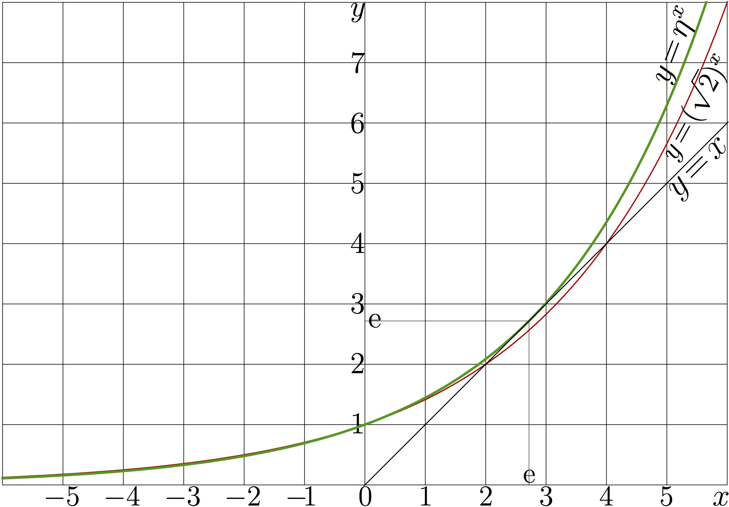 | 2,515 × 1,751 (350 KB) | Maintenance script (talk | contribs) | Importing image file |
You cannot overwrite this file.
File usage
The following page uses this file: